This Fact Page displays text and images related to global warming and climate change
(Hover your mouse over the text below to "popup" a window with a related text.
Click on the text or image to open a new window with a detailed description.)

Figure 2.Climate and immunity correlations with annual state WNND cases. Figure 3.Climate, immunity and WNND cases. Keeping the Temperature Rise to 1.5° C Table 2.2 | The assessed remaining carbon budget and its uncertainties. Drought and immunity determine the intensity of West Nile virus epidemics and climate change impacts Figure 2.Climate and immunity correlations with annual state WNND cases. The effect of (a) immunity (cumulative incidence; coeff. = -2.05, F1,300 = 96.42, p < 0.001), (b) precipitation (coeff. = -0.0009, F1,161 = 2.20, p = 0.14), (c) drought (coeff. = -0.14, F1,274 = 27.01, p < 0.001), (d) winter severity (coeff. = -0.05, F1,34 = 2.95, p = 0.09), (e) temperature (PIP: coeff. = 0.06, F1,276 = 2.58, p = 0.10; TAR: coeff. = 0.22, F1,144 = 53.59, p < 0.001; QUI: coeff. = 0.002, F1,104 = 0.0005, p = 0.98) and (f) temperature modelled as the relative R0 value at a given temperature (coeff. = 1.66, F1,121 = 17.33, p < 0.001) on the total logged number of WNND cases (adjusted for state random effects) in a given state and year (1999–2013). In (a–d,f), the filled red points and fitted lines are univariate regressions for states in which that predictor was significant (a < 0.05), while open black points depict states in which the predictor was not significant. In (e), green crosses, blue circles and green triangles denote states where C. tarsalis, C. pipiens and C. quinquefasciatus, respectively, dominate transmission and the relationship is only significant for C. tarsalis. (Online version in colour.) URL:     http://carbonbrief.us2.list-manage.com/track/click?u=39b25e6afa81d7ffc0e925ee9&id=ad7e6061a2&e=bf36e91829 Drought and immunity determine the intensity of West Nile virus epidemics and climate change impacts Figure 3.Climate, immunity and WNND cases. (a) Yearly WNND cases and fitted model (line) in nine representative states, and projections of the number of future cases under mean (M) or extreme (E—95th percentile) climate conditions for either current (cross-hatch) or future (star) climate projections. Error bars include both the standard error of the mean projected values and the standard deviation of the residuals between current projected and actual values. (b) Colours/shading indicate the significant variables in the fitted models by state with pie-charts showing their relative importance. (c) Human WNND cases and abundance of infected mosquitoes in Colorado when all humans were naive (2003, filled points, coeff = 0.99, F1,175 = 173.1, p < 0.001) and in subsequent years (2004–2008, open points, coeff = 0.72, F1,787 = 285.5, p < 0.001). Variables were power transformed (1/4) to equalize leverage and linearize the relationship. 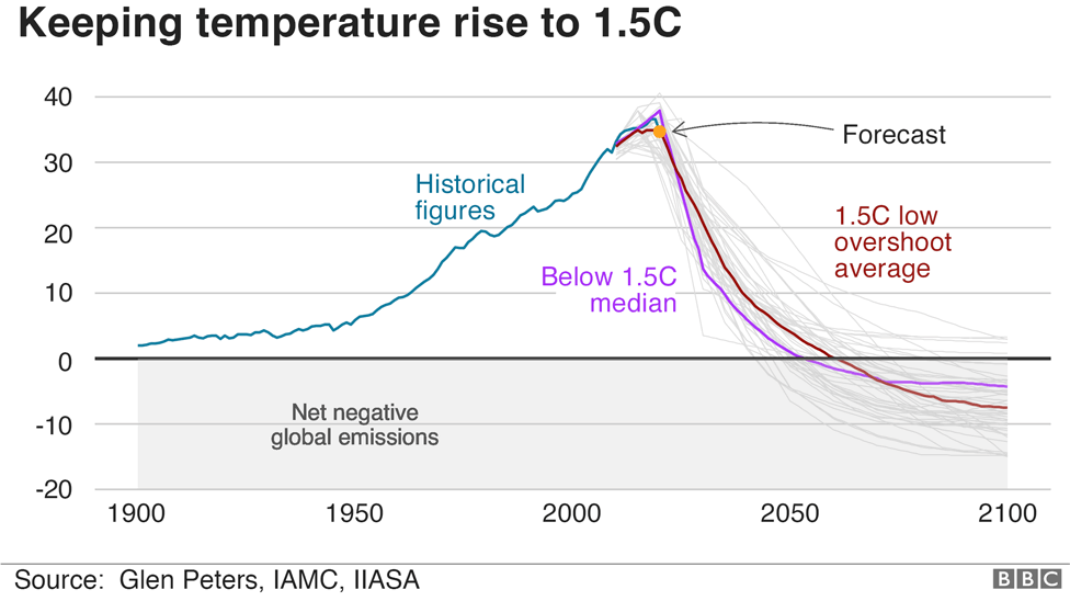(Online version in colour.) URL:     http://carbonbrief.us2.list-manage.com/track/click?u=39b25e6afa81d7ffc0e925ee9&id=ad7e6061a2&e=bf36e91829 Climate change and coronavirus: Five charts about the biggest carbon crash Keeping the Temperature Rise to 1.5° C "If Covid-19 leads to a drop in emissions of around 5% in 2020, then that is the sort of reduction we need every year until net-zero emissions are reached around 2050," said Glen Peters, also from Cicero. "Such emissions reductions will not happen via lockdowns and restrictions, but by climate policies that lead to the deployment of clean technologies and reductions in demand for energy." Energy experts believe there will be a bounce back next year, but that, long term, the world will move to greener fuels. URL:     https://www.bbc.com/news/science-environment-52485712 IPCC 1.5° C Report Table 2.2 | The assessed remaining carbon budget and its uncertainties. Shaded blue horizontal bands illustrate the uncertainty in historical temperature increase from the 1850–1900 base period until the 2006–2015 period as estimated from global near-surface air temperatures, which impacts the additional arming until a specific temperature limit like 1.5°C or 2°C relative to the 1850–1900 period. Shaded grey cells indicate values for when historical temperature increase is estimated from a blend of near-surface air temperatures over land and sea ice regions and sea-surface temperatures over oceans. Notes: *(1) Chapter 1 has assessed historical warming between the 1850–1900 and 2006–2015 periods to be 0.87°C with a ±0.12°C likely (1-standard deviation) range, and global near-surface air temperature to be 0.97°C. The temperature changes from the 2006–2015 period are expressed in changes of global near-surface air temperature. *(2) Historical CO2 emissions since the middle of the 1850–1900 historical base period (mid-1875) are estimated at 1940 GtCO2 (1640–2240 GtCO2, one standard deviation range) until end 2010. Since 1 January 2011, an additional 290 GtCO2 (270–310 GtCO2 , one sigma range) has been emitted until the end of 2017 (Le Quéré et al., 2018). *(3) TCRE: transient climate response to cumulative emissions of carbon, assessed by AR5 to fall likely between 0.8–2.5°C/1000 PgC (Collins et al., 2013), considering a normal distribution consistent with AR5 (Stocker et al., 2013). Values are rounded to the nearest 10 GtCO2 . *(4) Focussing on the impact of various key uncertainties on median budgets for 0.53°C of additional warming. *(5) Earth system feedbacks include CO2 released by permafrost thawing or methane released by wetlands, see main text. *(6) Variations due to different scenario assumptions related to the future evolution of non-CO2 emissions. *(7) The distribution of TCRE is not precisely defined. Here the influence of assuming a lognormal instead of a normal distribution shown. *(8) Historical emissions uncertainty reflects the uncertainty in historical emissions since 1 January 2011. URL:     https://www.ipcc.ch/site/assets/uploads/sites/2/2019/05/SR15_Chapter2_Low_Res.pdf